As we became more involved with water management, we realized that we needed a way to keep track of our progress. We decided that the best way to show the overall picture of our client's water use from year to year was to graph it. In cases where the client is not following our Water Management Program, their graphs show erratic water use throughout the years. By the same token several clients with charts reflecting the same level of water conservation suggests that clients are using a precise Program of Water Management.
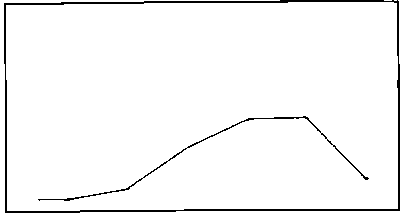
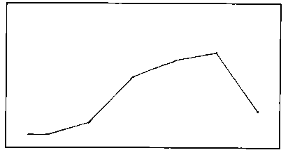
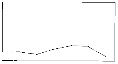
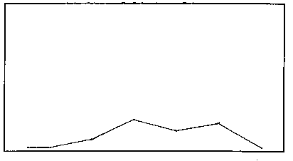
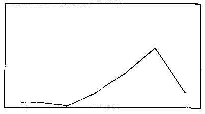
The graphs reflect one year of water use for each home during the drought years; 1987-1992. We divided the year up into two month blocks to simulate a water billing cycle. The center point between each month represents every other month. The measurement scale ranges from 10,000 gallons to 140,000 gallons of water.
Each of our clients had a consumption history one year prior to following our Water Management Program. We used those records as a base to compare our Water Management Program to. EBMUD provided our clients with the records and our clients then forwarded them to us. These graphs are based on accurate information. The graphed lines were determined by the water consumption records that were forwarded to us by our clients.
The figures are taken from our clients who reside in Alamo, Blackhawk, Danville, Moraga, and Walnut Creek. We've provided their names and addresses as well as what year their graph represents. We've also stated the approximate sizes of their lawn and landscape and whether they have a pool. As you read these charts you will see that water consumption varies greatly; some figures jump very high and some are very low. The reason for this is the simple fact that clients who have larger lawns use more water than those who have smaller lawns.
The graphs also show that water consumption varies according to the season. In January, February, November, and December, water use stabilizes because there is little to no outdoor water use. As we move into March, April, and May, we see that water usage increases slightly. At this point we are just beginning to turn on our outdoor water systems. As we move on to June, July, August, and September, we notice that water use is high. Daytime temperatures hover in the 90+ range most of the time. As daytime temperatures increase, the amount of water used increases. The summer also brings on a variety of hazzards to the irrigation system because the sprinklers are on for longer periods of time thus increasing the number of irrigation breaks that can occur. You'll notice that almost all the graphs show water usage peaking in September-October, during Contra CostaCounty's Indian Summer, when temperatures can soar up to 95 degrees and above. Immediately afterwards, we see water drop back down in November and December. By the end of October we usually get our first good rainfall.
Once we've received an inch of rain then we inform our clients that its time to turn off their automatic irrigation systems. They know that they can operate their systems manually for treatments or special circumstances. Years of water management have taught us that January, February, and March are critical times for encouraging the development of deeper root systems. Forcing our plants to hunt for their water source strenghtens them. At the same time it allows us to save water because we've turned off our irrigation systems. Compare that to a yard dependent upon its daily irrigation and a water bill so high that it skyrockets!

How To Read Our Graphs

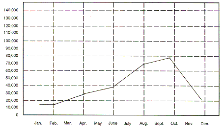
The graphs reflect one year of water use for each home during the drought years; 1987-1992. We divided the year up into two month blocks to simulate a water billing cycle. The center point between each month represents every other month. The measurement scale ranges from 10,000 gallons to 140,000 gallons of water.
Each of our clients had a consumption history one year prior to following our Water Management Program. We used those records as a base to compare our Water Management Program to. EBMUD provided our clients with the records and our clients then forwarded them to us. These graphs are based on accurate information. The graphed lines were determined by the water consumption records that were forwarded to us by our clients.
|
Customer 13 Blackhawk Graph Represents 1989 Lawn is approx. 800 sq. ft. Landscape is approx. under 10.000 sq. ft. | ||||||||
|
Customer 31 Blackhawk Graph Represents 1991 Lawn is approx. 3,950 sq. ft. Landscape is approx. over 10.000 sq. ft. Pool | ||||||||
|
Customer 33 Danville Graph Represents 1989 Lawn is approx. 536 sq. ft. Landscape is approx. under 10.000 sq. ft. | ||||||||
|
Customer 55 Walnut Creek Graph Represents 1992 There are no lawns Landscape is approx. over 10.000 sq. ft. Pool | ||||||||
|
Customer 56 Danville Graph Represents 1992 Lawn is approx. 256 sq. ft. Landscape is approx. over 10.000 sq. ft. | ||||||||

|
Customer 58 Danville Graph Represents 1991 Lawn is approx. 256 sq. ft. Landscape is approx. over 10.000 sq. ft. |